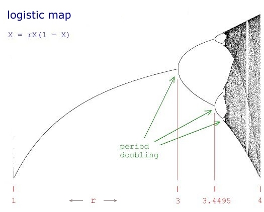
Logistic Map
The logistic map is the iterated discreet-value form
of the continuous-value logistic difference equation.
Mathematician Paul Stein called the complexity of
this iterated equation "frightening".
Computer program code format:
X = r * X * (1 - X)
which means:
X = r(previous X)(1 - previous X)
(Complete program code is at the bottom of page.)
This was Mitchell Feigenbaum's break-through
equation on his road to discovering universality
across different chaotic systems.
Iterating this equation produces regions of
distinct values, involving period doubling,
as well as regions of chaos. It is the rate of
convergence of period doubling that is universal.
Explanation:
A distinct set of values occur at a certain value
of r (r1). The number of distinct values suddenly
doubles at a higher value of r (r2). Take the
difference between r2 and r1. Divide that difference
by the difference between r3 (where the next doubling
occurs) and r2. That number (the convergence ratio)
approaches 4.6692016... as r increases. That
convergence ratio appears in many other chaotic
systems involving very different equations.
In this article, we present four ways in which
to graph this iterated equation in a static manner:
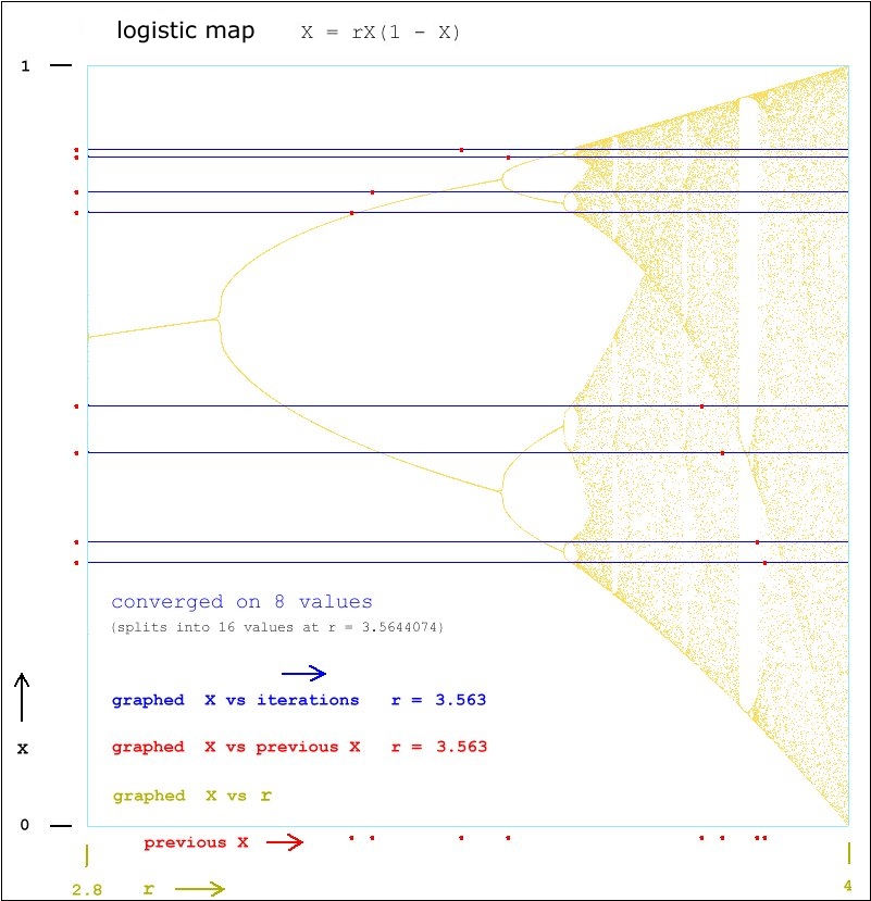
1. In a bifurcation diagram, the values of X are
plotted against the values of the parameter r.
One such diagram is shown at the top of this page.
2. Plotting X against the previous value of X for
a given value of r produces a parabolic curve,
always in segments corresponding to the range
of values that X acquires for that value of r.
Of special interest to investigators is the
question of whether a point lands to the left or
to the right of the previous point. Various
LRLRRRL patterns are found to repeat.
Below the diagrams section, there is a table
showing some L-R patterning and a table
showing L shift : R shift ratios for various
values of the parameter r.
(The shift ratio study is one of this author's
many original investigations/discoveries
regarding the logistic map. Six years later,
and this author still hasn't seen it discussed
anywhere else. - R.L. 11/28/22)
3. Plotting each value of X against each iteration
produces a straight line graph which reveals how
many iterations are needed for convergence to
distinct values for X for a given value of r.
(Anywhere from just a few iterations to four
million iterations prove to be sufficient,
depending on the value of r.)
4. Graphing in a circular manner: Plotting the
sine and cosine of an incrementally increasing
angle times the ever evolving X value reveals
hidden patterns amidst the chaotic zones.
All four types of graphs are displayed further down on
this page. (Types 3 and 4 are this author's creations.)
The initial value (0 - 1) for X makes no difference
in the appearance of any of the graphs. For some values
of r, the equation is sensitive to the initial value of
X, but the resulting values are not significantly
different from one initial value of X to another.
The range of values for r is 0 - 4.
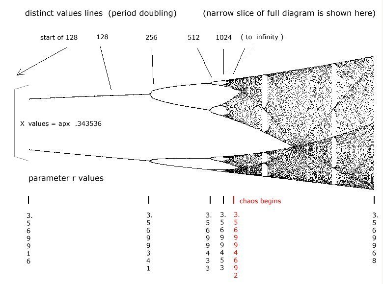
Here are some period doubling events for approximate
values of r:
distinct values r (range 0 - 4)
_______________ _________________
1 1
2 3
4 3.4494899
8 3.5440905
16 3.5644074
32 3.5687595
64 3.5696917
128 3.5698914
256 3.5699341
512 3.5699433
1024 3.5699453
2048 3.5699456
.
.
2^n 3.5699468376
and so on, without end as r approaches 3.56994692,
at which point chaos begins to take over.
The highest value of r below 3.56994692 for which
I discovered distinct values in the form 2^n was
3.5699468376. There must have been millions of
distinct values there.
Distinct values also appear when r > 3.56994692,
in between periods of chaos. For instance, one such
set is found at r = 3.57004996211.
Distinct values also occur in groups of
6, 12, 18, 24... and 5, 10... in this higher region.
(See notes below the graphs section for general
information about generating a bifurcation diagram.
Program code for all four diagram types follows that.)
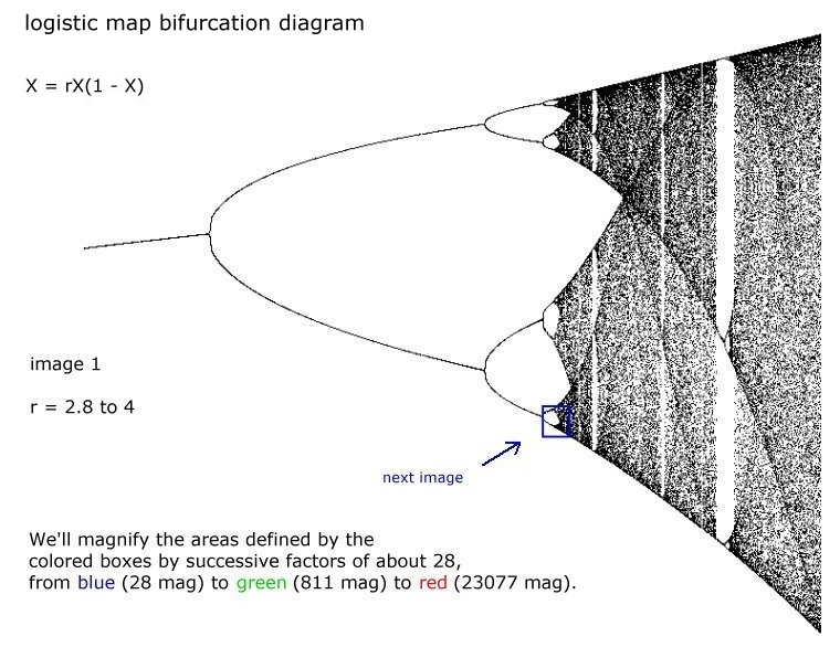
 ========================================================================
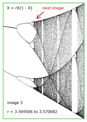
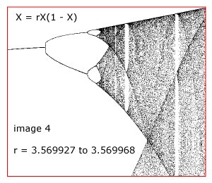
This algorithm is infinitely deep. Similar, yet never
identical, patterns repeat as one looks infinitely deeper.
After displaying the following four bifurcation
diagrams exploring the infinite depth of this algorithm,
we'll look at some graphs for single values of the
parameter r.
note:
Do you think it's easy to magnify a select area of
a mathematically generated image on a computer?
Guess again !
There are an abundance of issues, including the
mismatch of coordinate systems between programming
language and computer display, shift factors for
properly framing the target area, and on and on..
This author worked out the following formula in order
to easily facilitate progressive magnification
without having the image wildly disappear off
the screen:
YSHIFT = (((700*P)-760)*(-1)+([((P*(-1)*700*AMP)+760]*(-1)
end note
========================================================================
This algorithm is infinitely deep. Similar, yet never
identical, patterns repeat as one looks infinitely deeper.
After displaying the following four bifurcation
diagrams exploring the infinite depth of this algorithm,
we'll look at some graphs for single values of the
parameter r.
note:
Do you think it's easy to magnify a select area of
a mathematically generated image on a computer?
Guess again !
There are an abundance of issues, including the
mismatch of coordinate systems between programming
language and computer display, shift factors for
properly framing the target area, and on and on..
This author worked out the following formula in order
to easily facilitate progressive magnification
without having the image wildly disappear off
the screen:
YSHIFT = (((700*P)-760)*(-1)+([((P*(-1)*700*AMP)+760]*(-1)
end note
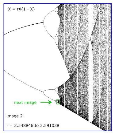
 ========================================================================
To appreciate just how abruptly chaos ends
and distinct value lines begin, see the
following diagram.
========================================================================
To appreciate just how abruptly chaos ends
and distinct value lines begin, see the
following diagram.
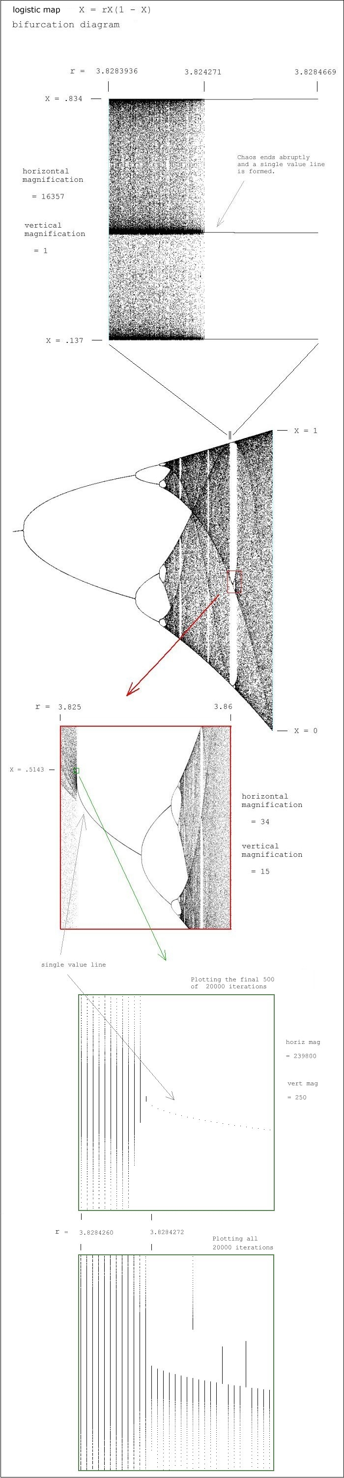
 Shown below are the final two X values out of twenty
thousand iterations for the middle distinct value
line for each value of r. See the graphs immediately
above.
As r approaches 3.8284272, the X values are
not yet stable (though they are becoming bunched
quite tightly), and they are not falling downwards
in an overall sense:
r X
3.8284268 .514396041025985
3.8284268 .514396756770264
3.8284269 .514516155621660
3.8284269 .514517495144266
3.8284270 .514118995580905
3.8284270 .514121155779832
3.8284271 .514407341511282
3.8284271 .514407484278966
Chaos ends (for awhile) at r = 3.824271
The .514... values are falling now and they are
locked in on a single value for each iteration
of the current parameter r:
3.8284272 .514288397179200
3.8284272 .514288397179200
3.8284273 .514253214008774
3.8284273 .514253214008774
3.8284274 .514227367177942
3.8284274 .514227367177942
3.8284275 .514205928117646
3.8284275 .514205928117646
The same is true for the other two distinct X value
lines at this value of r, as well as for any r value
splitting event.
=======================================================================
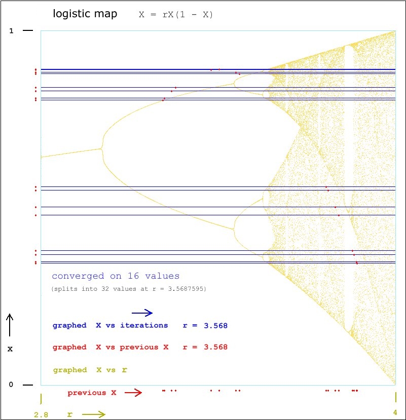
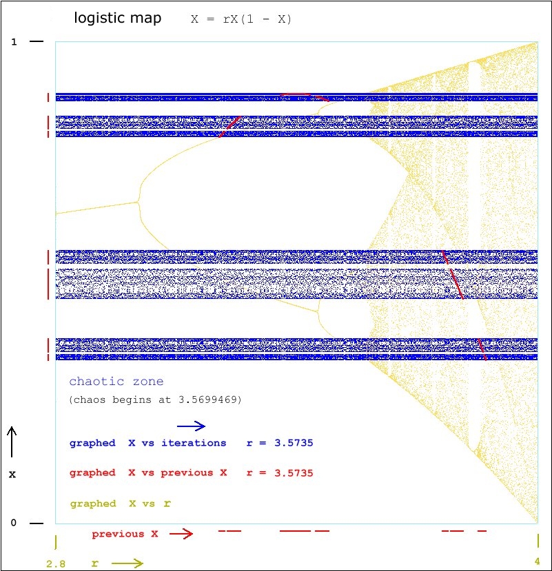
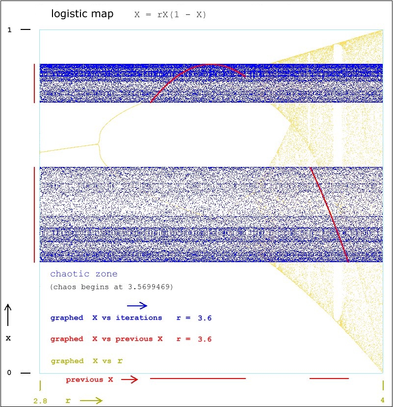
The following five images show the straight graphing
(X plotted against iterations in blue) and the parabolic
graphing (X plotted against the previous X in red)
superimposed onto a bifurcation diagram.
Note that the bifurcation diagram simply makes for an
interesting backdrop. Do not try to make correlations
beyond the match-up of the X values, which itself has
no significance.
Shown below are the final two X values out of twenty
thousand iterations for the middle distinct value
line for each value of r. See the graphs immediately
above.
As r approaches 3.8284272, the X values are
not yet stable (though they are becoming bunched
quite tightly), and they are not falling downwards
in an overall sense:
r X
3.8284268 .514396041025985
3.8284268 .514396756770264
3.8284269 .514516155621660
3.8284269 .514517495144266
3.8284270 .514118995580905
3.8284270 .514121155779832
3.8284271 .514407341511282
3.8284271 .514407484278966
Chaos ends (for awhile) at r = 3.824271
The .514... values are falling now and they are
locked in on a single value for each iteration
of the current parameter r:
3.8284272 .514288397179200
3.8284272 .514288397179200
3.8284273 .514253214008774
3.8284273 .514253214008774
3.8284274 .514227367177942
3.8284274 .514227367177942
3.8284275 .514205928117646
3.8284275 .514205928117646
The same is true for the other two distinct X value
lines at this value of r, as well as for any r value
splitting event.
=======================================================================
The following five images show the straight graphing
(X plotted against iterations in blue) and the parabolic
graphing (X plotted against the previous X in red)
superimposed onto a bifurcation diagram.
Note that the bifurcation diagram simply makes for an
interesting backdrop. Do not try to make correlations
beyond the match-up of the X values, which itself has
no significance.

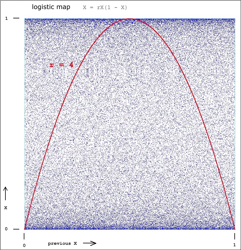
 Here is the only full parabola, that generated at r = 4:
 Here is some output showing RRRL patterning:
Note that the Rs and Ls indicate a right or left
shift from the previous plotted point, not the
direction of the point from the central axis.
X value shift
.3186, " R"
.7685129016, " R"
.6297689087271950, " R"
.8253865073602450, "L"
.5101976177307690, " R"
.8846318704178640, "L"
.3612864678763470, " R"
.8168852882604630, " R"
.5295263478576550, " R"
.881913809528948, "L"
.368662121002446, " R"
.823936279853100, " R"
.513531114546066, " R"
.884351857644560, "L"
.362048719319123, " R"
.817631832321111, " R"
.527849467601022, " R"
.882254401326362, "L"
.367740767239850, " R"
.823076533537926, " R"
.515500299308996, " R"
.884149482153514, "L"
.362599280778603, " R"
.818168489945347, " R"
.526641594500876, " R"
.882487398066276, "L"
.367110001734535 " R"
.822484479197956, " R"
.516853312794537, " R"
.883994519101387, "L"
==================================================
The ratio of total L shifts to total R shifts for
a given value of r can take on many values,
such as
0:1
1:1
1:2
1:2.333...
1:3
1:4
1:4.333...
1:5
1:6
1:7
and, we surmise, other ratios as well.
(One can already detect a pattern -- with the .333..
decimal portion following powers of 2 in the right
side of the ratios.)
These ratios remain uniform over specific ranges of r.
These ratios do not correlate with the number of distinct
value lines. I found examples of the L:R ratio
changing in the midst of a range of a given number
of distinct values.
Between r = 3.56994687 and 3.56994693, the
L:R ratio alternates between two distinct values:
1:5.04723799963414
and
1:5.04724714191982
This is the exact region of r where period
doubling of the 2^n variety ends and chaos begins.
This may be the only region where recurring values
of L:R ratios are found that are not tidy ratios.
Here is a tiny snapshot of the L:R ratios going through
some changes through adjacent ranges of r:
total total L:R
init X r L shifts R shifts ratio iterations
------ ------ -------- -------- ------- ----------
".90"," 3.7416," ",200000," ",800000," ",0," ",4," ",1000000," ",0
".90"," 3.7417," ",200000," ",800000," ",0," ",4," ",1000000," ",0
".90"," 3.7418," ",200000," ",800000," ",0," ",4," ",1000000," ",0
".90"," 3.7419," ",300000," ",700000," ",0," ",2.3333," ",1000000," ",0
".90"," 3.7420," ",300000," ",700000," ",0," ",2.3333," ",1000000," ",0
".90"," 3.7421," ",300000," ",700000," ",0," ",2.3333," ",1000000," ",0
".90"," 3.7422," ",300000," ",700000," ",0," ",2.3333," ",1000000," ",0
".90"," 3.7423," ",300000," ",700000," ",0," ",2.3333," ",1000000," ",0
".90"," 3.7424," ",300000," ",700000," ",0," ",2.3333," ",1000000," ",0
".90"," 3.7425," ",300000," ",700000," ",0," ",2.3333," ",1000000," ",0
".90"," 3.7426," ",300000," ",700000," ",0," ",2.3333," ",1000000," ",0
".90"," 3.7427," ",300000," ",700000," ",0," ",2.3333," ",1000000," ",0
".90"," 3.7428," ",250000," ",750000," ",0," ",3," ",1000000," ",0
".90"," 3.7429," ",250000," ",750000," ",0," ",3," ",1000000," ",0
Interesting patterns appear when graphing chaotic zones
in a circular manner, running sufficient iterations to
complete hundreds of orbits.
(These same patterns are generated by at least two
other very different algorithms. One is the Balloting
algorithm seen on another page of this website. Another
is a repeating line drawing routine used to color a
plane in a CAD program. That image is also displayed on
the Balloting page. These patterns cannot be generated
by simply orbiting random numbers -- an algorithm is
required.)
Here is a graph generated at r = 3.59
Here is some output showing RRRL patterning:
Note that the Rs and Ls indicate a right or left
shift from the previous plotted point, not the
direction of the point from the central axis.
X value shift
.3186, " R"
.7685129016, " R"
.6297689087271950, " R"
.8253865073602450, "L"
.5101976177307690, " R"
.8846318704178640, "L"
.3612864678763470, " R"
.8168852882604630, " R"
.5295263478576550, " R"
.881913809528948, "L"
.368662121002446, " R"
.823936279853100, " R"
.513531114546066, " R"
.884351857644560, "L"
.362048719319123, " R"
.817631832321111, " R"
.527849467601022, " R"
.882254401326362, "L"
.367740767239850, " R"
.823076533537926, " R"
.515500299308996, " R"
.884149482153514, "L"
.362599280778603, " R"
.818168489945347, " R"
.526641594500876, " R"
.882487398066276, "L"
.367110001734535 " R"
.822484479197956, " R"
.516853312794537, " R"
.883994519101387, "L"
==================================================
The ratio of total L shifts to total R shifts for
a given value of r can take on many values,
such as
0:1
1:1
1:2
1:2.333...
1:3
1:4
1:4.333...
1:5
1:6
1:7
and, we surmise, other ratios as well.
(One can already detect a pattern -- with the .333..
decimal portion following powers of 2 in the right
side of the ratios.)
These ratios remain uniform over specific ranges of r.
These ratios do not correlate with the number of distinct
value lines. I found examples of the L:R ratio
changing in the midst of a range of a given number
of distinct values.
Between r = 3.56994687 and 3.56994693, the
L:R ratio alternates between two distinct values:
1:5.04723799963414
and
1:5.04724714191982
This is the exact region of r where period
doubling of the 2^n variety ends and chaos begins.
This may be the only region where recurring values
of L:R ratios are found that are not tidy ratios.
Here is a tiny snapshot of the L:R ratios going through
some changes through adjacent ranges of r:
total total L:R
init X r L shifts R shifts ratio iterations
------ ------ -------- -------- ------- ----------
".90"," 3.7416," ",200000," ",800000," ",0," ",4," ",1000000," ",0
".90"," 3.7417," ",200000," ",800000," ",0," ",4," ",1000000," ",0
".90"," 3.7418," ",200000," ",800000," ",0," ",4," ",1000000," ",0
".90"," 3.7419," ",300000," ",700000," ",0," ",2.3333," ",1000000," ",0
".90"," 3.7420," ",300000," ",700000," ",0," ",2.3333," ",1000000," ",0
".90"," 3.7421," ",300000," ",700000," ",0," ",2.3333," ",1000000," ",0
".90"," 3.7422," ",300000," ",700000," ",0," ",2.3333," ",1000000," ",0
".90"," 3.7423," ",300000," ",700000," ",0," ",2.3333," ",1000000," ",0
".90"," 3.7424," ",300000," ",700000," ",0," ",2.3333," ",1000000," ",0
".90"," 3.7425," ",300000," ",700000," ",0," ",2.3333," ",1000000," ",0
".90"," 3.7426," ",300000," ",700000," ",0," ",2.3333," ",1000000," ",0
".90"," 3.7427," ",300000," ",700000," ",0," ",2.3333," ",1000000," ",0
".90"," 3.7428," ",250000," ",750000," ",0," ",3," ",1000000," ",0
".90"," 3.7429," ",250000," ",750000," ",0," ",3," ",1000000," ",0
Interesting patterns appear when graphing chaotic zones
in a circular manner, running sufficient iterations to
complete hundreds of orbits.
(These same patterns are generated by at least two
other very different algorithms. One is the Balloting
algorithm seen on another page of this website. Another
is a repeating line drawing routine used to color a
plane in a CAD program. That image is also displayed on
the Balloting page. These patterns cannot be generated
by simply orbiting random numbers -- an algorithm is
required.)
Here is a graph generated at r = 3.59
 Shrinking the image to 1/2 size, previously unseen
strong patterns appear:
Shrinking the image to 1/2 size, previously unseen
strong patterns appear:
 At 1/3 size:
 Another one at r = 3.64
 1/2 size:
 1/3 size:
 Here is r = 3.64 again, superimposed on another
pattern which we discuss on another page:
Here is r = 3.64 again, superimposed on another
pattern which we discuss on another page:
 Finally, at r = 3.9 we see another chaos zone:
 Notes about generating bifurcation diagrams:
The standard way to generate this diagram is to use a nested
loop. The outside loop iterates values of incremented r
and resets the value of X to its initial value. The inside
loop iterates the equation.
Interestingly, one can also generate a bifurcation diagram by
using just a single loop, whereby r is incremented for
each iteration of the equation.
The resulting diagram is nearly indistinguishable from the
one obtained using the nested loop algorithm. Looking
closely, one can detect a slight difference in the dots
comprising the chaotic zones, and examining the data read out
reveals that period doubling events are slightly off. For
example, period two occured at about 3.004, as opposed to 3.
The code:
(X in some of the program code is not the same X that appears
in the equation appearing on this page or in the discussion
on this page. Rather, it is the horizontal axis plot value.)
============================================================
My Visual BASIC program code for the bifurcation diagram:
Private Sub bifurbtn_Click()
viewport.ScaleMode = pixel
viewport.DrawWidth = 1
'viewport.Line (80, 60)-(780, 60), RGB(148, 234, 252) 'top
'viewport.Line (80, 760)-(780, 760), RGB(148, 234, 252) 'bottom
'viewport.Line (80, 60)-(80, 760), RGB(148, 234, 252) 'left
'viewport.Line (780, 60)-(780, 760), RGB(148, 234, 252) 'right
'viewport.Line (430, 60)-(430, 760), RGB(148, 234, 252) 'center
yshift = Val(yshiftbox.Text)
'xshift = val(xshiftbox.text)
amp = Val(dsamp.Text)
If amp = 0 Then amp = 1
ITER = Val(itera.Text)
If ITER = 0 Or ITER > 1000 Then ITER = 1000
reset# = Val(numb.Text)
If reset# = 0 Then reset# = 0.9
expand = Val(expandbox.Text)
If expand = 0 Then expand = 1
ri# = Val(parameter.Text)
If ri# = 0 Then ri# = 2.8
rf# = Val(rfbox.Text)
If rf# = 0 Or rf# > 3.999 Then rf# = 3.999
range = CInt((rf# - ri#) * 583.333 * expand)
X = (583.33 * (ri# - 2.8)) + 80
rinc# = 0.0017143
If expand > 1 Then X = 80: rinc# = rinc# / expand
r# = ri#
For g = 1 To range
num# = reset#
r# = r# + rinc#
X = X + 1
For a = 1 To ITER
num# = r# * num# * (1 - num#)
Y# = (-num# * 700 * amp) + 760 + yshift
viewport.PSet (X, Y#), RGB(0, 0, 0)
100:
Next a
Next g
totalpoints = g * a
xplotbox.Text = " "
xplotbox.Text = Str$(g)
totalptsbox.Text = " "
totalptsbox.Text = Str$(totalpoints)
rincbox.Text = " "
rincbox.Text = Str$(rinc#)
finalrbox.Text = " "
finalrbox.Text = Str$(r#)
finalnum.Text = " "
finalnum.Text = Str$(num#)
End Sub
===========================================================
My Visual BASIC program code for bifurcation listing values:
Private Sub quick2loopbtn_Click()
ITER = Val(itera.Text)
reset# = Val(numb.Text)
If reset# = 0 Then reset# = 0.9
rinc# = 0.0000001 ' or whatever
r# = 3.8284151 ' or whatever
For g = 1 To 80
num# = reset#
r# = r# + 0.0000001
For a = 1 To 4000000 ' or whatever
num# = r# * num# * (1 - num#)
If a <= 999990 Then GoTo 100
Open "ds\" + "list2" + ".txt" For Append As #1
Write #1, r#; " "; num#
Close #1
100:
Next a
Open "ds\" + "list2" + ".txt" For Append As #1
Write #1, " "
Close #1
Next g
g = g - 1: a = a - 1
totalpoints = g * a
xplotbox.Text = " "
xplotbox.Text = Str$(g)
totalptsbox.Text = " "
totalptsbox.Text = Str$(totalpoints)
rincbox.Text = " "
rincbox.Text = Str$(rinc)
finalrbox.Text = " "
finalrbox.Text = Str$(r)
finalnum.Text = " "
finalnum.Text = Str$(num#)
End Sub
============================================================
My Visual BASIC program code for the parabola version:
Private Sub parabtn_Click()
viewport.ScaleMode = pixel
viewport.DrawWidth = 1
viewport.Line (80, 60)-(780, 60), RGB(148, 234, 252) 'top
viewport.Line (80, 760)-(780, 760), RGB(148, 234, 252) 'bottom
viewport.Line (80, 60)-(80, 760), RGB(148, 234, 252) 'left
viewport.Line (780, 60)-(780, 760), RGB(148, 234, 252) 'right
'viewport.Line (430, 60)-(430, 760), RGB(148, 234, 252) 'center
dw = Val(drawwidthbox.Text)
If dw = 0 Then dw = 1
viewport.DrawWidth = dw
ITER = Val(itera.Text)
If ITER = 0 Then ITER = 100000
r = Val(parameter.Text)
para$ = parameter.Text
X# = Val(numb.Text)
If X# = 0 Then X# = 0.9
RR = 0
LL = 0
pt5 = 0
For a = 1 To ITER
Y# = r * X# * (1 - X#)
If a < 50000 Then GoTo 50
TEMPX# = (700 * X#) + 80
TEMPY# = (-700 * Y#) + 760
viewport.PSet (TEMPX#, TEMPY#), RGB(255, 0, 0)
viewport.PSet (TEMPX#, 770), RGB(255, 0, 0) ' shows previous X values
viewport.PSet (70, TEMPY#), RGB(255, 0, 0) ' shows X values
50:
X# = Y#
Next a
statusbox.Text = "done"
End Sub
============================================================
My Visual BASIC program code for the parbola L:R listing version:
Private Sub quickparabtn_Click()
ITER = Val(itera.Text)
If ITER = 0 Then ITER = 20000
r# = Val(parameter.Text)
para$ = parameter.Text
rinc# = Val(rincbox.Text)
loops = Val(gbox.Text)
resetx# = Val(numb.Text)
init$ = numb.Text
If X# = 0 Then X# = 0.9: init$ = ".90"
RR = 0
LL = 0
pt5 = 0
oops = 0
For g = 1 To loops
X# = resetx#
r# = r# + rinc#
For a = 1 To ITER
Y# = r# * X# * (1 - X#)
'If a < 999000 Then GoTo 50
'Open "ds\" + "xy-list" + ".txt" For Append As #1
'Write #1, init$; " "; r#; " "; X#; " "; Y#
'Close #1
If X# = 0.5 Then pt5 = pt5 + 1: GoTo 50
If Y# < X# And X# > 0.5 Then sh$ = " R": RR = RR + 1
If Y# > X# And X# > 0.5 Then sh$ = "L": LL = LL + 1
If Y# < X# And X# < 0.5 Then sh$ = "L": LL = LL + 1
If Y# > X# And X# < 0.5 Then sh$ = " R": RR = RR + 1
50:
X# = Y#
Next a
If LL = 0 Then LL = 1: oops = oops + 1 ' prevents division by zero
LRRATIO# = RR / LL
Open "ds\" + "lr-ratio" + ".txt" For Append As #1
Write #1, init$; " "; r; " "; LL; " "; RR; " "; pt5; " ";
LRRATIO#; " "; ITER; " "; oops; " "; X#; " "; Y#
Close #1
RR = 0
LL = 0
pt5 = 0
oops = 0
Next g
statusbox.Text = "done"
End Sub
============================================================
My Visual BASIC program code for the straight graph version:
Private Sub logdifstrbtn_Click()
viewport.ScaleMode = pixel
viewport.DrawWidth = 1
viewport.Line (80, 60)-(780, 60), RGB(148, 234, 252) 'top
viewport.Line (80, 760)-(780, 760), RGB(148, 234, 252) 'bottom
viewport.Line (80, 60)-(80, 760), RGB(148, 234, 252) 'left
viewport.Line (780, 60)-(780, 760), RGB(148, 234, 252) 'right
'viewport.Line (430, 60)-(430, 760), RGB(148, 234, 252) 'center
r# = Val(parameter.Text)
amp = Val(dsamp.Text)
If amp = 0 Then amp = 1
inc = Val(dsinc.Text)
If inc = 0 Then inc = 0.007
num# = Val(numb.Text)
If num# = 0 Then num# = 0.9
ITER = Val(itera.Text)
If ITER = 0 Then ITER = 100000: inc = 0.007
yshift = Val(yshiftbox.Text)
X = 80
For a = 1 To ITER
num# = r# * num# * (1 - num#)
X = X + inc
Y# = (-num# * 700 * amp) + 760 + yshift
viewport.PSet (X, Y#), RGB(0, 0, 255)
Next a
finalnum.Text = " "
finalnum.Text = Str$(num#)
End Sub
============================================================
My Visual BASIC program code for the circular graph version:
Private Sub logisticrunbtn_Click()
R = Val(parameter.Text)
num# = Val(numb.Text)
ra = Val(radiusmult.Text) * 450
ITER = Val(itera.Text)
anginc# = Val(angleinc.Text) * (3.14159265358979 / 180)
For a = 1 To ITER
num# = R * num# * (1 - num#)
angle# = angle# + anginc#
X# = num# * (Cos(angle#) * ra) + 430
Y# = num# * 1.2284 * (Sin(angle#) * ra) + 530
viewport.PSet (X#, Y#), RGB(0, 0, 0)
Next a
finalnum.Text = " "
finalnum.Text = Str$(num#)
End Sub
=============================================================
home
Balloting
Simple trig
Logistic map
The Attractor of Henon
Number doubling
Barnsley's Fern
The Sierpinski Triangle
Notes about generating bifurcation diagrams:
The standard way to generate this diagram is to use a nested
loop. The outside loop iterates values of incremented r
and resets the value of X to its initial value. The inside
loop iterates the equation.
Interestingly, one can also generate a bifurcation diagram by
using just a single loop, whereby r is incremented for
each iteration of the equation.
The resulting diagram is nearly indistinguishable from the
one obtained using the nested loop algorithm. Looking
closely, one can detect a slight difference in the dots
comprising the chaotic zones, and examining the data read out
reveals that period doubling events are slightly off. For
example, period two occured at about 3.004, as opposed to 3.
The code:
(X in some of the program code is not the same X that appears
in the equation appearing on this page or in the discussion
on this page. Rather, it is the horizontal axis plot value.)
============================================================
My Visual BASIC program code for the bifurcation diagram:
Private Sub bifurbtn_Click()
viewport.ScaleMode = pixel
viewport.DrawWidth = 1
'viewport.Line (80, 60)-(780, 60), RGB(148, 234, 252) 'top
'viewport.Line (80, 760)-(780, 760), RGB(148, 234, 252) 'bottom
'viewport.Line (80, 60)-(80, 760), RGB(148, 234, 252) 'left
'viewport.Line (780, 60)-(780, 760), RGB(148, 234, 252) 'right
'viewport.Line (430, 60)-(430, 760), RGB(148, 234, 252) 'center
yshift = Val(yshiftbox.Text)
'xshift = val(xshiftbox.text)
amp = Val(dsamp.Text)
If amp = 0 Then amp = 1
ITER = Val(itera.Text)
If ITER = 0 Or ITER > 1000 Then ITER = 1000
reset# = Val(numb.Text)
If reset# = 0 Then reset# = 0.9
expand = Val(expandbox.Text)
If expand = 0 Then expand = 1
ri# = Val(parameter.Text)
If ri# = 0 Then ri# = 2.8
rf# = Val(rfbox.Text)
If rf# = 0 Or rf# > 3.999 Then rf# = 3.999
range = CInt((rf# - ri#) * 583.333 * expand)
X = (583.33 * (ri# - 2.8)) + 80
rinc# = 0.0017143
If expand > 1 Then X = 80: rinc# = rinc# / expand
r# = ri#
For g = 1 To range
num# = reset#
r# = r# + rinc#
X = X + 1
For a = 1 To ITER
num# = r# * num# * (1 - num#)
Y# = (-num# * 700 * amp) + 760 + yshift
viewport.PSet (X, Y#), RGB(0, 0, 0)
100:
Next a
Next g
totalpoints = g * a
xplotbox.Text = " "
xplotbox.Text = Str$(g)
totalptsbox.Text = " "
totalptsbox.Text = Str$(totalpoints)
rincbox.Text = " "
rincbox.Text = Str$(rinc#)
finalrbox.Text = " "
finalrbox.Text = Str$(r#)
finalnum.Text = " "
finalnum.Text = Str$(num#)
End Sub
===========================================================
My Visual BASIC program code for bifurcation listing values:
Private Sub quick2loopbtn_Click()
ITER = Val(itera.Text)
reset# = Val(numb.Text)
If reset# = 0 Then reset# = 0.9
rinc# = 0.0000001 ' or whatever
r# = 3.8284151 ' or whatever
For g = 1 To 80
num# = reset#
r# = r# + 0.0000001
For a = 1 To 4000000 ' or whatever
num# = r# * num# * (1 - num#)
If a <= 999990 Then GoTo 100
Open "ds\" + "list2" + ".txt" For Append As #1
Write #1, r#; " "; num#
Close #1
100:
Next a
Open "ds\" + "list2" + ".txt" For Append As #1
Write #1, " "
Close #1
Next g
g = g - 1: a = a - 1
totalpoints = g * a
xplotbox.Text = " "
xplotbox.Text = Str$(g)
totalptsbox.Text = " "
totalptsbox.Text = Str$(totalpoints)
rincbox.Text = " "
rincbox.Text = Str$(rinc)
finalrbox.Text = " "
finalrbox.Text = Str$(r)
finalnum.Text = " "
finalnum.Text = Str$(num#)
End Sub
============================================================
My Visual BASIC program code for the parabola version:
Private Sub parabtn_Click()
viewport.ScaleMode = pixel
viewport.DrawWidth = 1
viewport.Line (80, 60)-(780, 60), RGB(148, 234, 252) 'top
viewport.Line (80, 760)-(780, 760), RGB(148, 234, 252) 'bottom
viewport.Line (80, 60)-(80, 760), RGB(148, 234, 252) 'left
viewport.Line (780, 60)-(780, 760), RGB(148, 234, 252) 'right
'viewport.Line (430, 60)-(430, 760), RGB(148, 234, 252) 'center
dw = Val(drawwidthbox.Text)
If dw = 0 Then dw = 1
viewport.DrawWidth = dw
ITER = Val(itera.Text)
If ITER = 0 Then ITER = 100000
r = Val(parameter.Text)
para$ = parameter.Text
X# = Val(numb.Text)
If X# = 0 Then X# = 0.9
RR = 0
LL = 0
pt5 = 0
For a = 1 To ITER
Y# = r * X# * (1 - X#)
If a < 50000 Then GoTo 50
TEMPX# = (700 * X#) + 80
TEMPY# = (-700 * Y#) + 760
viewport.PSet (TEMPX#, TEMPY#), RGB(255, 0, 0)
viewport.PSet (TEMPX#, 770), RGB(255, 0, 0) ' shows previous X values
viewport.PSet (70, TEMPY#), RGB(255, 0, 0) ' shows X values
50:
X# = Y#
Next a
statusbox.Text = "done"
End Sub
============================================================
My Visual BASIC program code for the parbola L:R listing version:
Private Sub quickparabtn_Click()
ITER = Val(itera.Text)
If ITER = 0 Then ITER = 20000
r# = Val(parameter.Text)
para$ = parameter.Text
rinc# = Val(rincbox.Text)
loops = Val(gbox.Text)
resetx# = Val(numb.Text)
init$ = numb.Text
If X# = 0 Then X# = 0.9: init$ = ".90"
RR = 0
LL = 0
pt5 = 0
oops = 0
For g = 1 To loops
X# = resetx#
r# = r# + rinc#
For a = 1 To ITER
Y# = r# * X# * (1 - X#)
'If a < 999000 Then GoTo 50
'Open "ds\" + "xy-list" + ".txt" For Append As #1
'Write #1, init$; " "; r#; " "; X#; " "; Y#
'Close #1
If X# = 0.5 Then pt5 = pt5 + 1: GoTo 50
If Y# < X# And X# > 0.5 Then sh$ = " R": RR = RR + 1
If Y# > X# And X# > 0.5 Then sh$ = "L": LL = LL + 1
If Y# < X# And X# < 0.5 Then sh$ = "L": LL = LL + 1
If Y# > X# And X# < 0.5 Then sh$ = " R": RR = RR + 1
50:
X# = Y#
Next a
If LL = 0 Then LL = 1: oops = oops + 1 ' prevents division by zero
LRRATIO# = RR / LL
Open "ds\" + "lr-ratio" + ".txt" For Append As #1
Write #1, init$; " "; r; " "; LL; " "; RR; " "; pt5; " ";
LRRATIO#; " "; ITER; " "; oops; " "; X#; " "; Y#
Close #1
RR = 0
LL = 0
pt5 = 0
oops = 0
Next g
statusbox.Text = "done"
End Sub
============================================================
My Visual BASIC program code for the straight graph version:
Private Sub logdifstrbtn_Click()
viewport.ScaleMode = pixel
viewport.DrawWidth = 1
viewport.Line (80, 60)-(780, 60), RGB(148, 234, 252) 'top
viewport.Line (80, 760)-(780, 760), RGB(148, 234, 252) 'bottom
viewport.Line (80, 60)-(80, 760), RGB(148, 234, 252) 'left
viewport.Line (780, 60)-(780, 760), RGB(148, 234, 252) 'right
'viewport.Line (430, 60)-(430, 760), RGB(148, 234, 252) 'center
r# = Val(parameter.Text)
amp = Val(dsamp.Text)
If amp = 0 Then amp = 1
inc = Val(dsinc.Text)
If inc = 0 Then inc = 0.007
num# = Val(numb.Text)
If num# = 0 Then num# = 0.9
ITER = Val(itera.Text)
If ITER = 0 Then ITER = 100000: inc = 0.007
yshift = Val(yshiftbox.Text)
X = 80
For a = 1 To ITER
num# = r# * num# * (1 - num#)
X = X + inc
Y# = (-num# * 700 * amp) + 760 + yshift
viewport.PSet (X, Y#), RGB(0, 0, 255)
Next a
finalnum.Text = " "
finalnum.Text = Str$(num#)
End Sub
============================================================
My Visual BASIC program code for the circular graph version:
Private Sub logisticrunbtn_Click()
R = Val(parameter.Text)
num# = Val(numb.Text)
ra = Val(radiusmult.Text) * 450
ITER = Val(itera.Text)
anginc# = Val(angleinc.Text) * (3.14159265358979 / 180)
For a = 1 To ITER
num# = R * num# * (1 - num#)
angle# = angle# + anginc#
X# = num# * (Cos(angle#) * ra) + 430
Y# = num# * 1.2284 * (Sin(angle#) * ra) + 530
viewport.PSet (X#, Y#), RGB(0, 0, 0)
Next a
finalnum.Text = " "
finalnum.Text = Str$(num#)
End Sub
=============================================================
home
Balloting
Simple trig
Logistic map
The Attractor of Henon
Number doubling
Barnsley's Fern
The Sierpinski Triangle

|